The most frequent question about Delphi programming I got was "How do you create these textures in your software Buttonz and Tilez?". Well, I am not going to release the source code, but here's an article that should explain the basics.
 
You can also download a sample project for D2 (should compile with higher versions, tough...) with some more optimized code, examples of how to use functions together, and a simple implementation of perlin noise.
 

 
1. Gradients:
 
I can almost hear you cry "Gradients are sooo easy, what do they do in this article?" -well... Most gradient implementations I have seen in Delphi so far were created using the most basic way: They have a start value (Tcolor) and an end value. However, much more flexible gradients can be created using a sinus function.
 
The big advantage is that we can change the frequency, and so get as many transitions as we want within the target area. A minor drawback is that, when not properly coded, this might be slighlty slower on old CPUs. The pseudo-code for a horizontal gradient would be:
 

freq_temp:=image.width / frequency; with image.canvas do for y:=0 to image.width do for x:=0 to image.height do begin z:=trunc(abs(sin(x/freq_temp*pi)*255)); pixels[x,y]:=rgb(z,z,z); end;

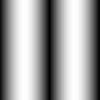The variable freq_temp is used to determine the number of transitions (or stripes). To understand this, have a look at the following graphs which show a sinus-curve at different frequencies (drawn very stupidly with Delphi ):
 

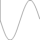y:=64+trunc(sin(x/64*pi)*64);

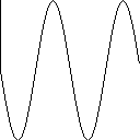
y:=64+trunc(sin(x/32*pi)*64);

 
2. Sinus Plasma:
 
A common effect in so called "demos" is the interference plasma: Three or more sinus functions which are overlapped to produce a texture. If you have some knowledge of physics, you might know overlapping sinus waves give a new wave, called interference (I hope this is expressed this way in english). If you take several functions which are depended of either x, y or both, you'll get a nice texture.
 

for y:=0 to image.width do for x:=0 to image.height do begin z1:=sin(x/freq_temp*1.7*pi); z2:=sin((x/3+y)/freq_temp*1.5*pi); z3:=sin(y/freq_temp*0.9*pi); {almost any variation will give interesting results} z:=trunc(abs(z1+z2+z3)*255); pixels[x,y]:=rgb(z,z,z); end;

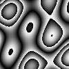 When playing with the frequency in this example, you will notice that the frequency can be compared to a "zoom level" - voila, we've get a texture that can be easily scaled! This effect can also be misused for simple animation effects. Together with color cycling, it really looks psychadelic... :)
 

 
3. Cellular Automats:
 
Interesting textures can also be created by applying some rules of growth to a matrix, just like in the classic "game of life". Cellular automats & reaction-diffusion patterns are, however, extremly complex topics and so I've only added a very simple example here. It starts of with an array of random values, and calculates the average of each value and it's eight neighbours, and finally add 1 to that average. Though the result is interesting, it really takes some time - the image depicted here has taken 2000 iterations to render. Of course, modifying the rules can give much more interesting images.
 

for i:=0 to iterations do for x:=1 to 254 do for y:=1 to 254 do array1[x,y]:= ((array2[x-1, y-1]+array2[x+1, y-1]+ array2[x-1, y+1]+array2[x+1, y+1]+ array2[x-1, y] +array2[x+1, y]+ array2[x, y-1] +array2[x, y+1]+ array2[x, y]) div 9)+1;

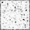As you can see in the code, I used two arrays that represents the image for the rendering. The first array starts of with random noise, and sort of a median cut as repeatedly applied to the image.
 

 
4. Plasma Clouds (aka Cubic Plasma):
 
The "Plasma Cloud" algorithm is my fave for 2 reasons: It renders much more quickly than, for example, reaction diffusion patterns, and also produces very nice and flexible images.
 
They are generated by a recursive algorithm that randomly puts values to the corners of a rectangle (squares are preferred, however), and then continues recursively quartering the whole rectangle until there are no zero values left. Random colors are averaged with the delta of a point so that small neighborhoods do not show much change, for a smoothed-out effect:
 

XA,YA] --- NewValue --- [XB,YB] Points A and B are known to be non-zero. The new Value would therefor be : (plasma[xa,ya]+plasma[xb,yb])/2 +(random-0.5)*(Abs(xa-xb)+Abs(ya-yb))

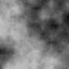You can see that the average of the two original points is calculated, and a random value that depends on the distance of the two original pixels is added. This value can also be used to control the "noisyness" of the final image. Tip: you can get seamless results by pre-rendering the outer lines of the image and mirroring them!